

Expect to hear increasing buzz around graph neural network use cases among hyperscalers in the coming year. Behind the scenes, these are already replacing existing recommendation systems and traveling into services you use daily, including Google Maps.
For those who remember paper maps and the unpredictability of navigating new cities, few trips go by that we do not silently thank the magical forces guiding us to our destination. And for longer journeys, few of us have not tried mightily to beat the projected ETA, often with success as a two or three-minute improvement, despite best efforts.
ETA services aren’t all about our individual convenience. Accurate ETA predictions are used globally to determine shipping routes and to reroute fleets on a dime if needed. The stakes are high — and so is the complexity of delivering accurate, fast transit guidance.
Other than giving us an appreciation how little difference going eight miles an hour over the speed limit makes, that ETA service is a remarkable invention — and one that takes a hell of a lot of compute power to achieve, if the graph neural network training efforts of Alibaba, Amazon, and Snapchat are any guide. On the systems side, data access is irregular, sparsity is king, and memory issues abound, which means training massive graphs, even on the world’s largest systems, comes with some major challenges. With that said, the improvements appear to be making graph neural networks worth the trouble and expense, as results below will show.
This week we gathered insight into how Google Maps provides ETA predictions in production. While graph neural networks (GNNs) are challenging to deploy at scale, this particular workload demands them over other traditional HPC or earlier-stage graph efforts.
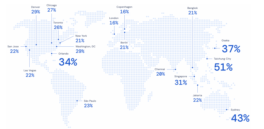
Google needs to factor the roads, driving conditions, historical and emerging traffic events. Arriving at this graph neural network destination took the combined work of Google as well as Amazon, Waymo, and Sea AI Lab, but now provides Google Maps with a far more accurate ETA and the ability to work with complex layers of data. The result for users is as much as a 40 per cent reduction in negative ETA outcomes in major cities like Sydney.
Predicting travel time has long been a holy grail for the transportation industry, certainly well before neural networks. But algorithmic sophistication and hardware never quite matched up enough until more recently to blend static and real-time data.
The Google Maps deployment builds on several pieces of work, including the baseline Graph Network framework. The tricky part was adding in spatiotemporal graph representation learning techniques, which have been developed over the last few years.
The problem, as with all GNNs, is in keeping fidelity in large-scale training. Accuracy is hard to maintain because the models are so large and complex, the only way to train them is by dividing them into segments or batches. Introducing that kind of split can create problems in convergence. Like the few other companies (Amazon and Alibaba are the best examples) training GNNs at webscale for production workloads, this has taken quite a bit of wrangling. Even still, latency, uncertainties, and range/coverage of the model are still outstanding issues.
Just as we pointed out in a recent article on Amazon’s challenges scaling GNN training, the Google mapping team says “ETA prediction in production invites particularly unstable training conditions across many batches of queries, particularly over routes of different scales.”
New frameworks like Graph WaveNet, ST-GRAT, StemGNN, and other research-focused efforts gave the collaborators sufficient methodologies to add richer spatiotemporal layers along with dynamic graph representation learning techniques that aid in richer topological featurization. The collaborators add that they have also looked at work at Baidu, where traffic predictions are also powered by GNNs.
All ETA predictions are the result of “supersegments” which are sequences of connected road segments that have predictable traffic flows. The moment you leave, the model already knows how long you’ll travel on each of those segments. And when you type in directions, it’s essentially a string of such segments served up sequentially. The interesting bit is in that sequence: the first is used to predict the next, and so on. “This lets us provide accurate travel time estimates in a scalable way, taking into account both spatial and temporal information,” the GNN team says.
In production Google says it’s using over a million of these supersegments. In the graph, each node is a road segment with edges where two segments connect. Models are regional in nature. The traversal times along segments and supersegments are denoted in seconds and those are used as node and graph-level labels for prediction. Each supersegment might appear in the training set multiple times as well since it’s the core of many separate paths. “Road segments are on average 50–100 meters long and the supersegments contain on average around 20 segments,” according to Google.
All of these segments are added into the model and, on serving, real-time information is also integrated, blending the moment with historical data for time of day/day of week.
“On a segment (node) level, we provide the average real-time and historical segment travel speeds and times, as well as segment length and segment priority (eg, road classifications such as highways) as features. On a supersegment (graph) level, we additionally provide real-time supersegment travel times as a feature. Real-time travel speeds and times are provided for 17 two-minute windows prior to horizon 0.” The researchers add that they also have learnable segments and supersegment-level embedding vectors. “This enables sharing of information whenever the same segment appears in different supersegments, and whenever the same supersegment appears in different candidate routes.”
Along the way, the training bottleneck was the high variability of the models, especially since models saved at different points during the training run were likely to result in variations in ETA results for different users. The team used a MetaOptimizer that uses MetaGradients (both developed at Google/DeepMind) that allows Google to tune the learning rate during the run while using approximation methods for some of the parameters during inference.
Google, like others in the literature we’ve linked here, is working to get graphs to take an extra step in pulling even more wisdom from node neighbors. In the Google Maps case, it is trying to use “extended supersegments” or even larger graphs that pull from nodes in neighboring segments, in addition to the original segments that might have other related traffic implications. “This enables our models to make use of additional spatial context — such as traffic congestion on a connecting route — at the expense of data storage, slower training, and inference.” The researchers add that the same GNN architecture is used for both supersegment and extended supersegment experiments, making the model storage cost remain constant and they are actively experimenting with binary features that indicate whether segments are on the main route in an extended graph.
Below is a sense of what these optimizations mean for your ETA. The percentages represent relative reduction in negative ETA outcomes compared to the prior approach used in production. A negative ETA outcome occurs when the ETA error from the observed travel duration is over some threshold and acts as a measure of accuracy.
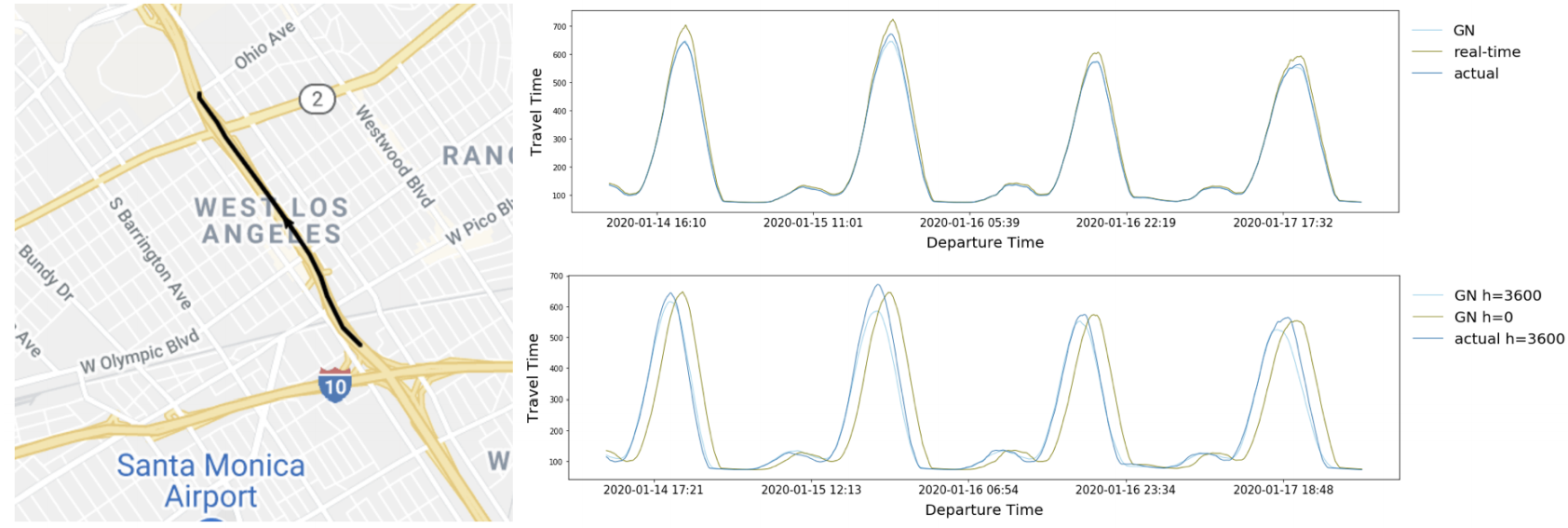
Below is an example of a supersegment in Los Angeles showing off the spatiotemporal advantages across different departure times from the airport — travel times and predictions over different departure times. “Our GNN is able to detect traffic congestions more accurately than using real-time travel times. Having multiple prediction horizons is important to providing accurate ETA,” Google says.
Even though what we would really like to know — exactly how much compute is required for the training of such graph neural networks, how often retraining is required, and what it costs Google to provide these ETAs — is not public, we can make some rough assumptions based on the experiences of the few other companies training GNNs at scale.
The thing to note about those experiences is that training beyond a certain point creates an unstable model with oversmoothing and huge resource consumption. The difference between ETA predictions and customer recommendations or other commercial uses of GNNs is that unlike recommendations or consumer demand, ETAs won’t change much with time outside of real-time inputs. Which could mean GNNs will remain at the core of Google Maps for a long time to come, and hopefully more optimizations at that scale can be shared.
The full model walkthrough is available here.


Be the first to comment