HexaMesh: Chiplet Topologies Inspired By Nature

With the reticle limit for chip manufacturing pretty much set in stone (pun intended) at 26 millimeters by 33 millimeters down to 2 nanometer transistor sizes with extreme ultraviolet lithography techniques and being cut in half to 26 millimeters by 16.5 millimeters for the High-NA extreme ultraviolet lithography needed to push below 2 nanometer transistor sizes, chiplets are inevitable and monolithic dies are absolutely going to become a thing of the past.

And so the question arises: When it comes to large complexes of chiplets, what is the best shape for a chiplet, and what is the optimal arrangement of these chiplets and the interconnects that link them together into a virtual monolith? (Again, pun intended.) Researchers at ETH Zurich and the University of Bologna played a little game of chiplet Tetris to try to find out, and came up with a neat configuration they call HexaMesh.

Engineering a chiplet interconnect topology is an engineering task that requires the balancing of a whole of constraints against a relative handful of absolute necessities – not an ideal situation at all. In such situations, all you can do is grin and bear the compromises you have to make. Torsten Hoefler, a professor at ETH Zurich, director of its Scalable Parallel Computing Laboratory (SPCL), chief architect for machine learning at the Swiss National Supercomputing Center, and a rising star in the HPC community, is one of the authors of the HexaMesh paper, which you can read here. One of his doctoral students, Patrick Iff, gave a presentation on the HexaMesh architecture, which you can watch here. We missed this one, and it came to our attention thanks to HPC Guru, so here is a tip of the hat to our well connected mysterious compatriot for pointing this out.

Given that so many components are on a mesh interconnect these days and every chip we have ever seen is rectangular, we have never given a lot of thought to the physical configurations of chiplets in a substrate package with 2.5D interposer connections. We had also assumed that the connections would be more or less like the NUMA links we see in server architectures. The more interconnect ports you put on a server CPU, the more tightly you can couple the CPUs into a shared memory system as well as the further you can scale that shared memory system. You can build a two-socket server, for instance, with just one link out of each server, but usually there are two so they can both tap each other’s memory. Three interconnect links per CPU means you can have four CPUs fully connected or eight CPUs with six out of eight of them having only one hop between the CPUs and two out of the eight requiring two hops.

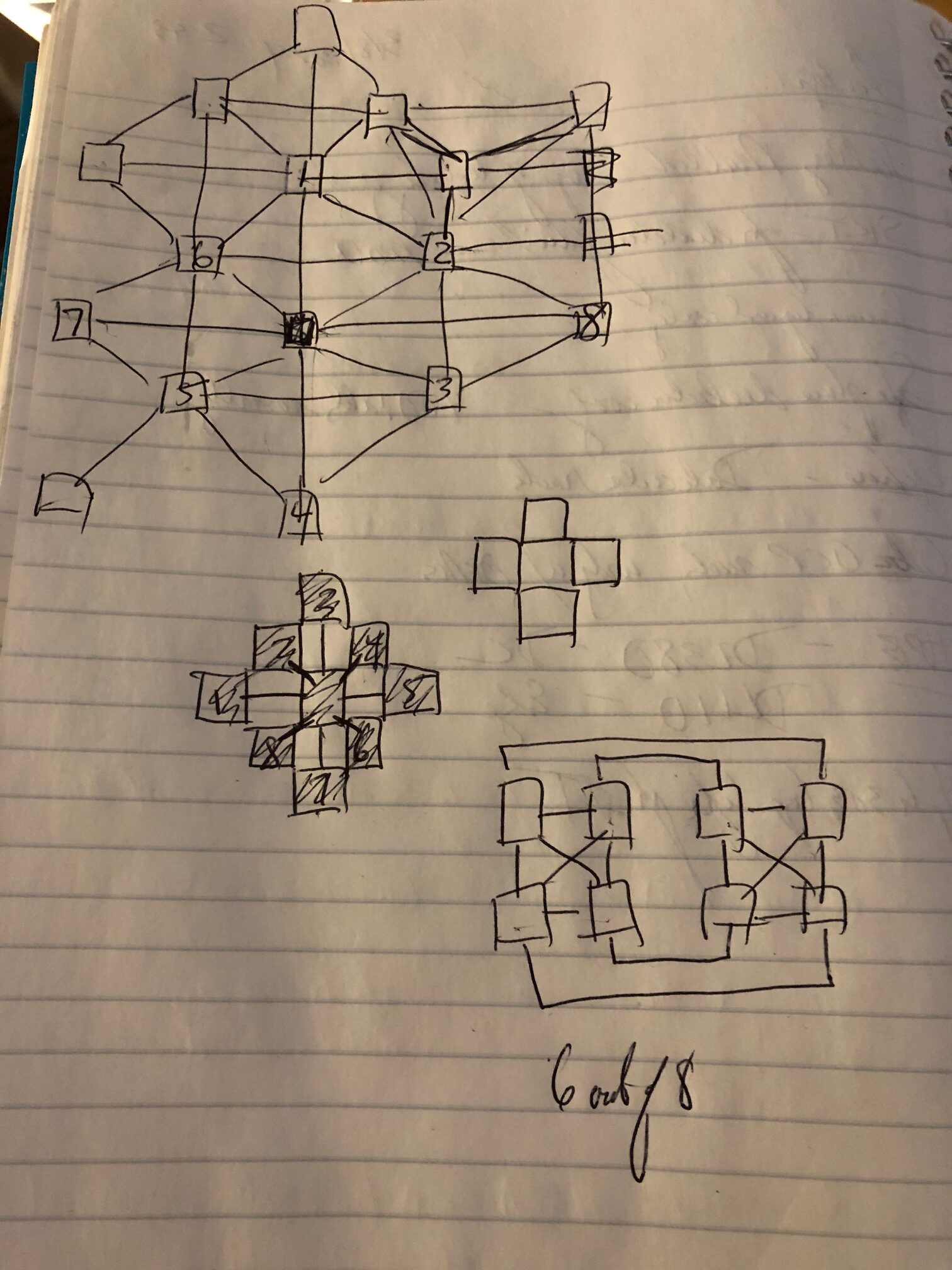
To build a mesh of chiplets, we would have just started with that quad building block, but bring eight ports out of each chiplet – one on each side and one out of each corner – to fully connect any chiplet to eight other nearby chiplets. Seems obvious, right?

We played around with some topologies and physical configurations, even spacing out the chiplets like a checkerboard square to try to make the links from the corners of the chiplets be the same length as the ones from the faces of the chiplets:

Not so fast, say the HexaMesh folks:

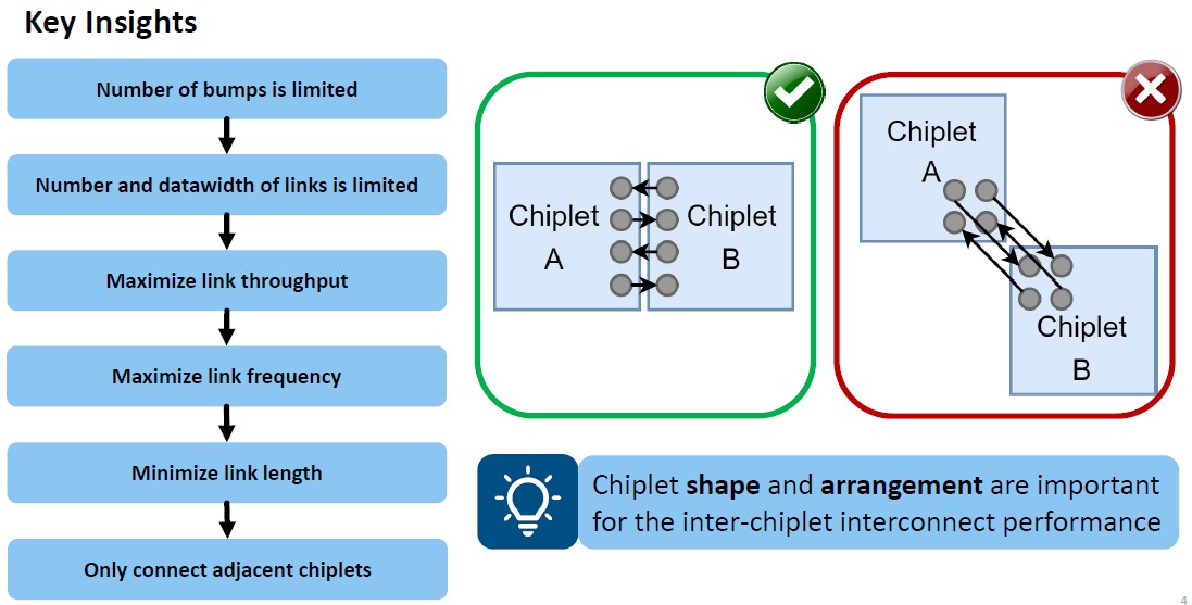
“To connect chiplets to the package substrate, controlled collapse chip connection (C4) bumps are used and to connect them to a silicon interposer, one uses micro-bumps,” they write in the paper. “The minimum pitch of these bumps limits the number of bumps per mm² of chiplet area, which limits the number and bandwidth of D2D links. As a consequence, D2D links are the bottleneck of the ICI. Since the D2D links limit the ICI data width, we want to operate them at the highest frequency possible to maximize their throughput. To run such links at high frequencies without introducing unacceptable bit error rates, we must limit their length to a minimum. The length of D2D links is minimized if we only connect adjacent chiplets. However, with such restricted connections, the shape and arrangement of chiplets has a significant impact on the performance of the ICI.”

OK, but our corner links coming out of the chiplets are direct connections, so we’re good with our theoretical OctoMesh approach, right? Wrong:

Chiplets apparently do not corner well.

We have also been told that we overvalue coherency. Which we always took as a compliment. . . . but perhaps not, especially here in the 21st century.

Anyway. The length of those corner-to-corner links are going to be much longer than on adjacent chiplets with faces that touch, and that means there will be higher error rates as well as higher latencies for those corner links. For NUMA machines there are definitely different latencies depending on the NUMA interconnect paths, and these can affect the performance of these shared memory machines to be sure. Most NUMA servers are partitioned in software in some fashion that makes workloads fit the physical hardware better, and the scaling is certainly not perfect for coherent memories. But as far as the HexaMesh creators are concerned, you can only have adjacent links and hope to have consistent high bandwidth and low latency with acceptable signal integrity.

Given all of this, the HexaMesh researchers came up with four different chiplet topologies and calculated the merits of each approach, and they are outlined below:

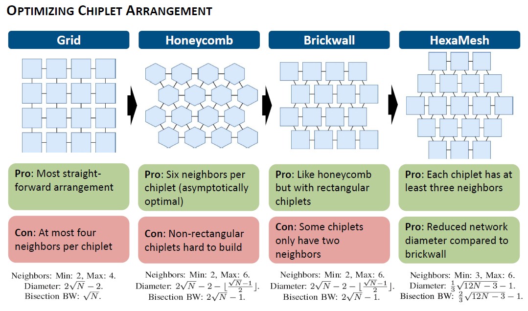
We added the math describing the range of neighbors in a mesh, the interconnect network diameter and bisection bandwidth for Grid, Honeycomb, Brickwall, and HexaMesh arrangements for chiplets on a 2.5D package to the presentation slide so you don’t have to go hunting around for it.

Don’t think about it for a second. Just look at the topologies above. Isn’t the Honeycomb topology so satisfying? But you can’t have non-rectangular chiplets because the machines that etch and cut chiplets do not like to do other shapes. Perhaps in the 22^nd century we will have such kind of chippery, and in three dimensions even like D&D die. . . . But look again. Isn’t the HexaMesh configuration solid, doesn’t it take the best of the Grid, Honeycomb, and Brickwall topologies and weave them into something, well, obvious once you see it? Building it out to a larger array of chiplets will show why your mind – if it is like our minds – really likes this HexaMesh configuration.

Here is what happens when you start with a seed couple of chiplets and then expand the chiplet cluster:

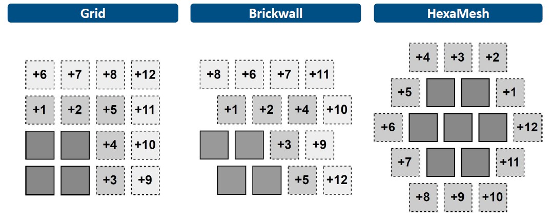
With the HexaMesh, you start at an indent and just do a circumference around the existing cluster, doing from seven core chiplets to a total of nineteen with the addition of a dozen more. This all assumes that the chiplets are the same size, of course.

While all of this is pretty mosaic work, what matters is how the die-to-die (D2D) interconnects perform, and to get an approximation of how this might look in the real world, the HexaMesh researchers ran some of the specs for the Universal Chiplet Interconnect Express, or UCI-Express, chip to chip interconnect through the BookSim2 simulator to see how the different chip topologies pan out. The model assumes a dozen wires per link and that the links operate at the 16 GHz upper limit of UCI-Express, which delivers 32 GT/sec data rates. With these and other inputs, scenarios were run for the four different chiplet arrangements, scaling from two to one hundred chiplets.

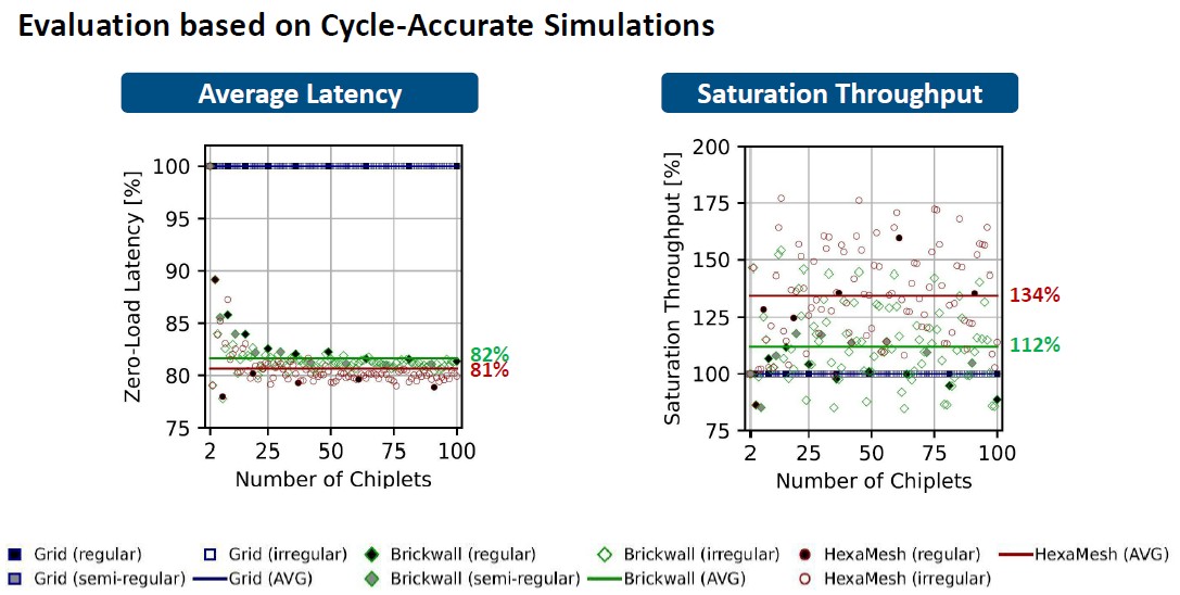
The performance of the different topologies in relation to each other varies as the number of chiplets scales up or down, but for more than ten chiplets, the Brickwall and HexaMesh reduce latency by 19 percent on average compared to the Grid, and the Brickwall delivers 12 percent higher bandwidth and the HexaMesh delivers 34 percent higher bandwidth. The network diameter of the HexaMesh setup is reduced by 42 percent compared to the Grid, and bi-section bandwidth for between ten and a hundred chiplets improves by 130 percent. And all done with rectangular chiplets that are standard in the industry.