The Nitty Gritty Of In Memory Computing

As noted at the beginning of this article series last week, an initial dive into in-memory computing meant questioning whether this was just another of those buzz words or whether there was some meat behind it. The meat might not be particularly fresh, but it seems that the way it is being prepared really is something new and novel.

We largely just need to agree on what all we are talking about when considering its use. Let’s start with column stores. Suppose that you have a massive database of customer information from throughout the world. But now you want to determine the opportunity to market to folks in, say, Rochester, Minnesota. You have built a similarly massive index of such customers over a table, because that buys you the opportunity quickly find Rochester-based customers and from there to only access the records of the customers from Rochester. The database manager obliges and bring into memory blocks of data which happen to include all of the information of all of those customers. Every single column of each of those customer’s records and more is brought into memory. Good. Indexes are/were a wonderful tool. But what did you really need? How much of even that was overhead?

Recall that it was read this way because the fields of each record were likely to have been contiguously packaged. In any given record (a row), the fields (the columns) of that record are often contiguously packaged out on disk and so in the DRAM. Said differently, the blocks that got read from disk contained complete records. But did your query need all that was accessed?  Or are you only interested in – say – the customer’s addresses?

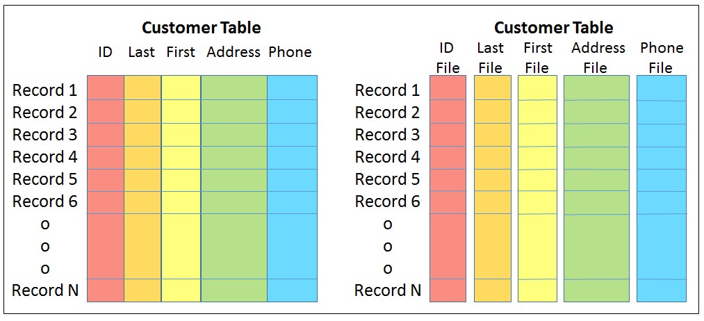
You didn’t care how your data is organized, only that it is accessible and available and secure.  So, let’s change things up. What if the contiguous data was the contents of the columns, not the contents of the rows?  Out on disk is your database table, organized today as arrays of rows, each row containing contiguous fields representing the columns.  Let’s change that to instead have the table consist of one-dimensional arrays, each consisting of only the contents of a column, each item of the column array being contiguous in memory with the next. Such a database table, instead, becomes a collection of such column-based data. At some level, this is a column-store, but it is more than that.

So, back to your search of folks from Rochester. The database manager reads the city/state column into memory and quickly scans this contiguous storage, noting the entries for Rochester. The remainder was not necessarily accessed. The read and the use of memory only involved this information.  Interestingly, the processor’s cache rather likes the array organization as well, so even such a scanning search for Rochester residents can be fast.

I present it this way largely to get the concept of a column store across, but it happens that an array – even though possibly arranged that way on disk – is not necessarily the fastest way to search for Rochester residents. I won’t take you on a trip through complex data structures here, but just know that any competent junior Computer Science major should know how to organize that data to make such a search faster still.

And here I get to a key point. We are talking about In-Memory Computing. The data as it resides on disk may really be this set of contiguous column-based arrays. But once brought into memory, is it a requirement that it stay organized that way?  Can it be organized “in-memory” in the way that your junior compsci major would prefer, perhaps even containing addresses?  Again, all you really care about – all your abstraction cares about – is that the data exists somewhere, somehow, and be secure and durable.  If there is a difference in organization at various steps, it just means that that abstraction needs to be transformed along the way, so when actually accessed – and frequently re-accessed – the in-memory data format provides for the most efficient execution.

I’ll add as a conclusion to this section, when a Computer Scientist uses the term “Load into memory”, they are not talking only about just reading bytes from a spinning disk into physical memory; they are referring to this entire process: Read into DRAM, map that into a Processes address space, and reorganize the file-based data into that of often complex objects for easy analysis.

Some Thoughts About Compression

As a bit of an aside, but this does get referenced as one of the tools in In-Memory Computing, we should mention the notion of data compression, especially as it relates to Column Stores.

The physical memory, although large, might still be smaller than the data that you want to wedge into it. And, getting something to fit easier or be loaded faster into processor cache improves performance as well. Data compression might be able to help.

Let’s start with a simple use case. Suppose your database table has a column representing a Boolean (i.e., True/False, Yes/No, Active/Inactive). You’ve defined the column as a character, thinking that only takes one byte per record and shoved the values ‘T’ or ‘F’ into that field. This is at least 8 bits and likely 16.

So now let’s define that Boolean column as a column store. On disk this might still be just a contiguous set of ‘T’ and ‘F’ characters. But, as a Boolean, it need only contain just one of two possible values. A number of you folks are reading this and saying “Hey, I can name that tune in 1 bit.” Yes you can. In memory this can be transformed into a simple bit array.  A 16 times compression. For a one-million record table, you just saved yourself about two megabytes of memory for another use.

Of course, to do this, we had to know that the column was compressible. This same case would not have been as compressible – if at all – if this information had been represented as a row-based table. There are all sorts of compression techniques, many are specialized like for word or name compression. Knowing the context, the right technique can be used.

Generic compression/decompression, though, takes time so this approach to saving memory must be taken as a trade-off. By that I mean that, in order to access the data in a compressed form, a decompression algorithm must first be executed. And there are essentially two ways to handle that:

1. Decompress the accessed data of the column with each and every access.
2. Decompress all or portions of the column – say individual pages – on first access. In this sense, rather than the compressed data being directly accessible by a processor, the compressed version of the data acts like another memory tier. One tier, albeit still in memory, is in the compressed format as it exists on disk. The second tier, also in memory, is the uncompressed version. It is the uncompressed version that is in the format usable by your program. Both exist in memory and both must be addressable somewhere. Changing the uncompressed version means recompressing if/when that data is to be returned to persistent storage. This takes time and memory.

And Now Remapping

Some In-Memory products make the point that having the database table in memory avoids the need for one or more associated indexes. Perhaps so; being in-memory would certainly allow for a more rapid scan than would be possible if it also meant reading from disk. But there are ways to represent data which are far more rapidly searched than even an in-memory table scan. In effect, it would be possible to avoid the traditional row/column-based table in memory as well.

To explain, even today you know that some of the data from a database table can reside within an Index. As such, for the right kind of query, the database table proper need not even be touched.

But suppose that we represented more than just one or two rows of a table in something like an index. Instead, let’s put everything otherwise found in a database table – or two or three – into a complex but more rapidly accessed data structure. And then let’s keep that data structure – call it an Index if you like – in memory. The row/column table, if it exists, does not get brought into memory. The content of the table on disk might still be in organized as row-and-columns (or not), but its contents have been remapped into something else – this complex data structure – in memory. In-memory, it might even contain the processor-friendly Effective Addresses if that allows for the fastest accesses.

As that remapped table’s contents gets changed, and the changes get logged, periodically even these changes can be written into the table proper on disk. Or not. If this complex structure contains all of the information (and does not contain Process-local Effective Addresses), perhaps this new data organization becomes what you understand to be a table object, but now also in persistent storage. The tables proper, after all, need not actually be organized physically as row-and-columns.

A Word About Pages

The system’s physical memory is typically organized as arrays of pages. It’s not that the physical memory cares at all; its virtual memory that requires this organizing unit. As outlined earlier, the total Virtual Address Space can be a lot larger than that of physical memory’s Real Address Space. Currently used pages of Virtual Address Space get mapped by the OS onto equal size pages of its Real Address Space; an OS-associated structure – we’ll call it a Page Table – in memory maintains this mapping.

There are a number of places that this matters to the performance of In-Memory Computing.

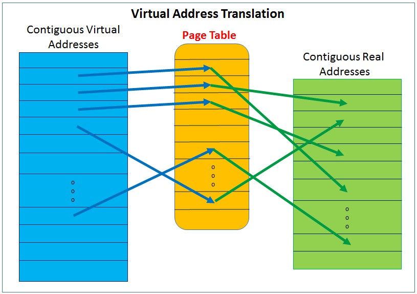
Each processor core’s hardware contains an “array” typically called a TLB (Translation Lookaside Buffer). Its purpose is to allow very rapid access of physical memory given an Effective/Virtual Address used by a program. It maps Virtual Addresses to Real Addresses.  Or more to the point, the core’s TLB maintains a small number of the virtual:real page mappings; these came from the OS’ Page Table. Only the TLB’s few mapped pages are accessible by the processor core at any moment in time.

The TLB is like a cache, but here the TLB is a cache of the page mappings otherwise maintained by the page table. If a program’s virtual address gets used and that virtual::real page mapping is not in the TLB, the program’s execution sort of stops until the TLB gets updated from the page table; time is passing and no work is getting done.

So why does this matter to In-Memory Computing?

First, even though the data is in memory, the processor hardware can’t access its pages until that page’s virtual::real page mapping is in the TLB.  The data is in memory, yes, but if that data is spread out over too many pages, say over more pages than can be held in the TLB, processing slows;  the processor is spending too much time updating the TLB rather than accessing data. Said differently, too many concurrently accessed pages can me slower execution.

So what can be done about it?  Part of the game, then, is the locality of your data. Again, even if your data is in memory, if the data actually being accessed in a period of time is in few enough pages to be represented in the TLB, processing can be fast. It not, if the same data is spread out over many more pages, processing can be slow (and anywhere in between). Improving the access locality to fewer pages can mean better performance.

Another technique is associated with page size. A number of processor architectures support a notion of large page(s). Their purpose is to allow more virtual memory to be mapped in the same number of TLB entries. For example, if the nominal page size is 4,096 bytes (which is typical), each aligned on a 4,096-byte boundary, a large page might be a few megabytes in size (for example, 16 MB on a 16 MB boundary). Given a TLB with 1K entries, 4K pages mean the processor core can have concurrent access to 4 MB; that same TLB with 16 MB pages can concurrently access 16 GB.

Large pages or not, the trick is packaging. Those objects being accessed together would best be served by residing in the same few pages. Given that the data objects require a lot of storage, the virtual pages used to hold these same objects might best be large pages. (Observe, though, that there is a trade-off here. If the entire virtual page is not being used, the associated physical storage is not being used either. If physical memory is being wasted, you can’t fit as much data into memory.)

In-Cache Computing

The apparently outrageous performance improvements claimed for In-Memory versus On-Disk data is certainly a function of the different access latencies. But in the same way that memory (DRAM) is multiple orders of magnitude faster than HDDs (and to a lesser extent I/O-based SSDs), it happens that the fastest processor cache (and TLB cache) is many orders of magnitude faster than DRAM memory. Given that memory can be accessed in half a microsecond; cache can often be accessed in better than half a nanosecond.

Similarly, as with programs not really accessing data on disk all of the time – a lot of data is both addressable and in DRAM memory some of the time – it happens that processors don’t access memory all of the time either. Processor cores actually only access data and instructions from their cache. If the needed data is not present there, the processor hardware transparently reads data blocks from the DRAM and into the cache. In a way, DRAM is to disk as cache is to DRAM.

So the trick in enabling the best possible In-Memory performance is both to arrange for the data to be in memory AND to arrange to maximize the in-cache hits (which – oddly, for a discussion on In-Memory Computing – means conversely minimizing the frequency of DRAM accesses). As you can imagine, cache optimization can be a field of performance optimization in its own right. [11]

One trick being used encapsulates access to a set of objects by a single thread, and so to a single core, and so to that core’s cache. Rather than any thread via its call stack accessing an object from any core, a single thread on a single core acts as a provider of a service. That thread, once bound to a core, pulls its objects into that core’s cache, and there they remain. The service is fast because, not only is the data in memory, but it is in that processor’s cache. A further benefit comes from the fact that no inter-thread locking or synchronization is required. Fast, from an execution time point of view, yes, but keep in mind that this single-core service is the only provider.  Used too frequently or if single-threaded processing takes too long, this same “advantage” could instead become a source of queueing delays.

File Store Versus Backing Store

This next might be rather esoteric so I’ll keep this short. You’ve seen that to have data accessed while in memory, that data must be mapped in under Virtual/Effective address spaces. It happens, though, that there is a bit of a related trade-off. You need as much as you can to be mapped within an address space, but performance also degrades if you have too much mapped. Huh?  Right!

This effect helps explain the title for this section. Yes, you want as much of what you have in files – that is File Store, that which is otherwise out on IO-based persistent storage – available to your processors, which in turn requires it to be both in memory and address mapped. But, because of the potentially huge size of the virtual and effective address spaces, you can have much more data mapped in an address space than will fit in physical memory. Again, the physical memory might be a handful of terabytes, but the address spaces are large enough to support exibytes.

There is nothing new here, aside from today’s magnitude of size. This effect has existed since virtual addresses spaces became larger than physical memory. As I’ve said a number of times, this too is something that has been true for nearly forever. And there has been a solution there as well. The solution for that was Backing Store. All that Backing Store is/was is a distinct part of HDD space – HDD space often separate from file store – reserved for the purpose of holding addressable data which could not fit into physical memory. Again, more data was assigned to the Virtual Address space than could fit in memory; this overflow had to reside somewhere, so it gets placed into this Backing Store on disk. When the overflow pages are needed again, the OS pages them back into DRAM, trading it with something else, with the “something else” getting written to Backing Store.

That has worked well historically, but you want In-Memory Computing. Whether the data is in File Store (and not normally mapped with a virtual address) or in Backing Store (and mapped with a virtual address), it is still in slower storage. You want the data to be virtual addressable AND in DRAM.

You can find a nice write up on this in Wikipedia under Paging and a nice related SlideShare presentation on UNIX Memory Management here.

I should observe, though, that there is way to have data in File Store and concurrently in a virtual address space; this does not use Backing Store. That way is via Memory-Mapped Files [5][6][7].  The essence of this is that any byte of a file even on disk – once memory-mapped – can be referenced via a virtual address. If that addressed byte is not in memory, the OS finds the location of your data, and if not in memory, pages the referenced data into memory. Unlike Backing Store, in which both changed and unchanged pages are written to disk when in-memory space is unavailable, changed pages of a memory-mapped file are written back to the file itself when aged or forced out of memory; unchanged pages in memory are simply thrown away since the disk-based file still has the current data.

And If That’s Not Enough: Distributed And NUMA Shared Memory

For all the theory above, what really kicked off In-Memory Computing was the simple fact that you can get a lot of memory in a system at a more reasonable price. It’s now not unreasonable to be talking about 512 GB to 1 TB of memory per processor chip, and most have multiple processor chips. My gosh.

But we can never seem to get enough of a good thing and more uses for more memory keep popping up. Just has been happening for now a couple decades, the way that we’ve been getting the many multiple times more memory has been both

1. Through replicating relatively smaller distributed systems, using rapid inter-systems data movement (commonly called “Scale Out”), and
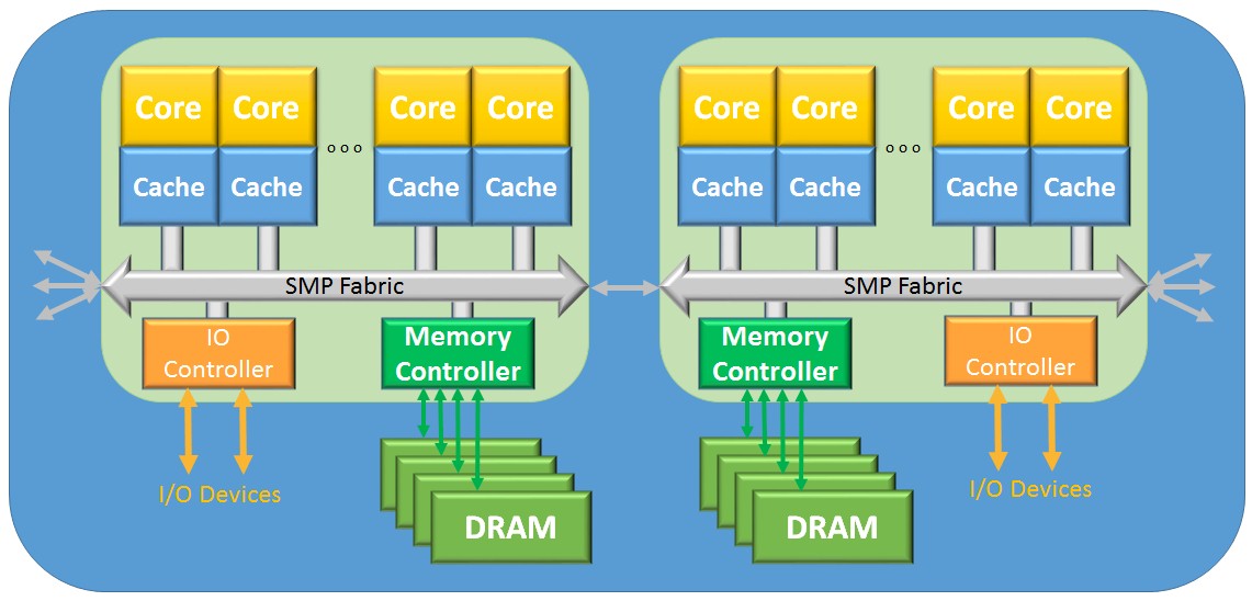
2. Through replicating the multi-core chips and their memory using a NUMA-based [8][9] (Non-Uniform Memory Access) SMP architecture, while maintaining the cache coherency and data sharing and simpler programming model found in the traditional SMP (commonly called “Scale Up”).

Many systems from both of these camps use the same basic building block, a multi-core processor chip with scads of DRAM per processor chip, and one or more different interconnects to IO space. Both types also group these into another form of building block consisting of one to a few such chips and memory, all chips maintaining a cache-coherent SMP single-system’s image; let’s here call this latter building block a “node.”

Using that node as a building block, the Scale-Out form expands using IO interconnects; PCI, Ethernet, InfiniBand, to name a few, using both point-to-point and switches of these protocols to grow. Memory, although immense, is also distributed and disjoint; data sharing between nodes must be done via I/O-based data copying, since the processors of one node cannot access the memory within remote nodes. For this reason, data sharing is inherently relatively infrequent.

The other, NUMA-based shared-memory systems allow any processor core to access any memory throughout the system, thereby simplifying the programming model. Such systems can consist of scads of nodes, and therefore also large amounts of shareable memory. The term NUMA comes from the fact that the access latency from some reference core is different based on the location of the DRAM being accessed; remote memory takes longer than local memory. The memory may all be sharable and cache-coherent, but if the rate of access to higher latency remote memory is not managed, applications are taking a hit on performance. Still, most multi-chip SMPs are NUMA-based, so some form of NUMA management should be considered increasingly the norm. The nodal interconnects after more proprietary than I/O interconnects since they support a cache-coherency protocol similar to that used within the nodes.

There are still other forms, another example includes systems which are NUMA-like – in the sense that processors can access all memory – but the contents of the cache is not necessarily kept coherent across all nodes.

At some level, stepping back a few feet, whether distributed or shared-memory, these systems look an awful lot like clustered systems built from the same building blocks, power supplies, and enclosures. One type is, though, and oddly, called “commodity systems.” The other, again oddly, is perceived – and often is priced – as expensive. And it’s this latter form which is easier to program and easier to manage. And it can offer superior performance when data sharing becomes – or must be – relatively frequent.

Driving the difference home, both types of systems can allow for the existence of a massive amount of DRAM for In-Memory Computing. Both types of systems also have some sort of a boundary between each of the “nodes” of those systems.

• The boundary between the distributed systems nodes, though, is hard; the processors of one node are incapable of accessing the memory of another. In such distributed systems, sharing of data between nodes implies explicit copying of that data from the DRAM of one to the DRAM of another. Wonderful things have been done over time to speed this process, but the boundary is real and noticeable from a performance point of view. The more frequent the need to share, the greater the impact of performance.
• On the other hand, for the NUMA-based systems, the boundary also exists but is also considerably softer, being more of a performance-based boundary. Sharing is enabled by the basic notion that a processor can access any of the memory within the entire system, even inter-node. Cache coherency is often maintained allowing a consistent and transparent view by all cores of the current data state. These systems can also be virtualized, perhaps for reasons of higher availability, with multiple operating system instances being packaged within a single system. Some of the NUMA latency issues can be managed by efficient placement of these OS instances within individual – or even set of particular – NUMA nodes.

An Addendum: In-Memory Computing And IBM i

When I first started reading up on In-Memory Computing, one of my first thoughts included “Yeah, but the IBM i OS has been capable of that for years.” Of course, there is more to IMC that just that, but I thought I’d share what lead me to that conclusion.

One of the many defining characteristics of the IBM i OS is its notion of a Single-Level Store (SLS). Rather than the two-step process of loading something in memory used by most OSes, every byte of data in IBM i has a virtual address from the moment the data is created. Every byte of even every persistent object is known by a unique virtual address value. And this remains true even if the OS is shut down and the power is off.

What makes this additionally Single-Level Store is that it does not matter whether that object being accessed is in DRAM or out on disk. If a program wants to access some object, it uses that object’s virtual address. Your program uses that object’s virtual address and the OS finds its location; if the object is not in DRAM, the OS transparently gets the object from its persistent storage location on disk. In such an addressing model, the DRAM is managed much like a cache for the contents of persistent storage like HDDs or SSDs.

Notice the key point here as it relates to IMC? Suppose that the DRAM available to your OS is about the size of your data working set. The database manager, for example, may ultimately use all of the database object’s virtual addresses; with every byte already addressed, all that happens is that the object’s pages are brought into the DRAM and – since there is plenty of space – left there. As with a cache, if the DRAM weren’t large enough, lesser used changed pages are written to disk. If the DRAM is large enough, even changed pages can remain in memory indefinitely; such changed data gets written back when it must be written back.

The notions of File Store and Backing Store don’t really exist either. There is, though, a notion of permanent and temporary segments of virtual address space; one continues across OS restarts, the other allows its storage to be reclaimed upon restart. In both any changed pages are written to the location of those virtual address segments on persistent storage. The permanent segments are used for anything that must persist. This includes files and DB tables, of course, but IBM i is also characterized as an “object-based” OS; all of the many types of objects that IBM i supports are also housed in one or sets of permanent segments. The temporary segments are used for at least stack and heap storage, but really generally as needed for non-persistent data.

More interestingly still, although IBM i also supports a notion of Process-Local Addressing, much of the SLS virtual address space is potentially common to all processes in the system. The same virtual address value means exactly the same thing to every process. As a result, data sharing is rather the norm. Of course, and correctly, some of you are saying “Hey, that violates basic security and integrity!” Interestingly, it doesn’t in this OS.  Perhaps someday The Next Platform will publish a more in depth article on IBM i and addressing; explaining here will take a while and this article has gotten too long as it is. But I will add that what they do with a variation on Capability Addressing – and its support within the hardware – might be useful in future systems.

Referenced Additional Reading

• [1] Statistic Brain … Average Historic Price of RAM, http://www.statisticbrain.com/average-historic-price-of-ram/
• [2] Memory Prices (1957-2015), http://www.jcmit.com/memoryprice.htm
• [3] 64-bit Computing … Wikipedia, https://en.wikipedia.org/wiki/64-bit_computing
• [4] … Power ISA Specification … See Virtual Address Generation section, https://www.power.org/documentation/power-isa-v-2-07b/
• [5] Memory-mapped file … Wikipedia, https://en.wikipedia.org/wiki/Memory-mapped_file
• [6] Managing Memory-Mapped Files, https://msdn.microsoft.com/en-us/library/ms810613.aspx
• [7] On Memory Mapped Files, http://ayende.com/blog/162791/on-memory-mapped-files
• [8] Non-uniform memory access … Wikipedia, https://en.wikipedia.org/wiki/Non-uniform_memory_access
• [9] NUMA (Non-Uniform Memory Access): An Overview, https://queue.acm.org/detail.cfm?id=2513149
• [10] In-Memory Big Data Management and Processing: A Survey
• [11] Locality of reference … Wikipedia, https://en.wikipedia.org/wiki/Locality_of_reference
• Implementation Techniques for Main Memory Database Systems
• How universal memory will replace DRAM, flash and SSDs
• ACID … (Atomicity, Consistency, Isolation, Durability) … Wikipedia, https://en.wikipedia.org/wiki/ACID
• Durability (database systems) … Wikipedia, https://en.wikipedia.org/wiki/Durability_(database_systems)
• Page (computer memory) … Wikipedia, https://en.wikipedia.org/wiki/Page_(computer_memory)
• UNIX Memory Management here … http://www.slideshare.net/Tech_MX/unix-memory-management